Creating Anisotropy Vector Fields from ROIs and Meshes
Creating vector fields of anisotropy can help determine associations between observed structural features and the mechanical function of a bone. With the property of being directionally dependent, anisotropy is presented as a 3D vector field in which color scales represent magnitude or direction and density is configurable. An example of a vector field computed for segmented trabecular bone is shown below.
Mapping of surface normal anisotropy by magnitude (on left) and direction (on right)

Dragonfly also provides a dedicated module for advanced bone analysis that includes a guided workflow with automated segmentation of cortical and trabecular bone, morphometric measurements, additional options for measurements of anisotropy, and volume fraction mapping (see Bone Analysis).
Right-click the required region of interest or mesh in the Data Properties and Settings panel and then choose 3D Modeling > Create an Anisotropy Vector Field to open the dialog shown below.
Create an Anisotropy Vector Field dialog

The following settings are available for creating anisotropy vector fields.
|
|
Description |
|---|---|
|
Algorithm |
The Surface normals algorithm is based on the construction of a surface mesh populated by a set of vectors perpendicular to the mesh faces with their magnitude being proportional to the local mesh face area. Note Refer to Mapping Methods and Settings for more information about the Surface normals algorithm. |
|
Sampling |
Lets you choose the sampling settings as follows: Area box… Defines the area for computing the vector field. Box shapes can be resized and/or reoriented as required (see Adding and Editing Shapes). You can also add multiple boxes to compute anisotropy in different orientations. Spacing… Determines the distance between the random points in the analysis area. You can also limit computations to a single voxel in the direction of the smallest length of the selected area box by checking the ‘Use single voxel in direction with smaller box length’ option. Grid size… Indicates the current grid size, which is computed as: area box length/spacing. |
| Neighbors |
Lets you choose the neighbors settings as follows: Radius of influence… Defines the kernel size, or elementary volume, within which anisotropy will be evaluated. You should note that a too small radius of influence may result in a low signal-to-noise ratio, while a too high radius can result in averaging and edge effects. Anisotropy evaluation… Lets you choose an evaluation method — Projection-based or Eigenvaluebased. You should note that both methods provide similar results, although you may find that the projection-based method is slightly more sensitive. |
| Mesh smoothing |
Determines the number of times that the mesh obtained from the input ROI will be smoothed before anisotropy is computed. Note Selecting one or two iterations usually provides for the most accurate results. |
-
Add a Box shape to the workspace and then adjust its size and/or orientation so that it defines the area for computing the vector field.
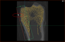
See Adding and Editing Shapes for information about working with shapes.
-
Right-click the required region of interest or mesh in the Data Properties and Settings panel and then choose 3D Modeling > Create an Anisotropy Vector Field.
The Create an Anisotropy Vector Field dialog appears.
-
Select the Sampling and Neighbors settings.
-
Select a number of iterations for mesh smoothing.
-
Click the Compute Scalar and Vector Fields button.
The vector field is added to the Data Properties and Settings panel when the computation is complete. You can examine the vector field in a 3D view (see Vector Field Properties and Settings).


